
Deep Reinforcement Learning for Automatic Stock Trading Bot
Keywords: Deep Reinforcement Learning, GRU, Attention Model, Encoder-decoder network

Abstract:
This project presented a new combination of Deep Reinforcement Learning algorithms. Prioritized Experience Replay which was proven to be robust in Atari Game revealed strong evidence to improve performance in the timeseries prediction task. In order to imitate the human-like learning instinct, Attention network was combined with encoding-decoding mechanism with the neural network to generate Q-values for the trading actions in this advanced DQN algorithm. Features including the long period of ema line and short period of ema line, MACD, RSI, volume, and time data were added together with the standised stock price to produce trading signals for the model. The new model was compared with traditional EMA strategies and RNN models with Evaluation Metrics including Sharpe Ratio, Win Ratio, Maximum Drawdown/Return and Annualized Return. Inspiring result was obtained when daily data was used.
Deep Q-Learning:
State and Action
The state design was one of the hardest tasks throughout the research. To concentrate on the research aims, the agent was set to only trade long and forbidden the short selling for simplicity reason. Also, the agent was only allowed to hold only one stock. In the replay memory, an additional column was added to show the holding stock status. A similar setting to (Gao X. 2019) of state and valid action pair was used.
Actions space: { ( 0 = Cash out or keep holding cash ), ( 1 = Buy a stock ) , ( 2 = keep holding a stock ) }
If the network output an invalid action, for example, when the agent was holding a stock, it was not supposed to buy another stock at the time. However, the network outputted 1 which violated the rule. In this case, the second highest value output would be chosen as the action.
Reward
Reward function was one of the vital elements to guide the agents to make correct decisions. By referencing to (Gao X. 2019), some amendments were made.
Rewards = { ( 0 = cash ) , (θ = Buy ) , ( σ = Sell ) }
where θ was the average price in the coming 5 timesteps less cost, σ was the price difference between next day price and current price.
The cost was defined as the current price multiply by a commission rate which was set at 0.25%. The reason to average out the price was based on the fact that the stock market was so noisy, and it was hard to predict one day movement. Averaging the price in future days as the target would be more feasible for the model as it would look into the future trend instead of short-term noisy movement.
Prioritized Experience Replay
Firstly, the Transition input was defined. It included the current state, action, next state, rewards and holding status. Each Transition was stored in the buffer. To rank each experience, the error from the loss function was used. The error was added an offset number to avoid too small error value. The probability of each transition would be equal to:\ Pr(i) = (p_i^α)/(∑p^α )
where p_i was equal to the error adding an offset number and α was the Alpha value for controlling the probability from too big which would dominate all other experience. For each sampling, the experience would be chosen randomly according to the probability distribution of the predefined probabilities. To increase the probability of the newly added experience, all the older experience probability would be deducted by the minimum probability from the replay memory. The weights were then estimated by the Equation (13). To be noted that, after each optimization, the priority list was updated.
Policy
To better strike a balance between exploration and exploitation, ε-greedy policy was used in this task.
Thresold=E+(S-E) e^((-step)/Decay)
where S= Start probability, E = End probability, step = step done in the loop, Decay is the decay time step. In each time step, a random number r∈[0,1] under uniform distribution were drawn. If the number is higher than the threshold in that step, the agent would choose to exploit which meant it would choose the action according to the output from the network, otherwise, the agent would choose to explore which meant it would randomly take an action regardless of the output of the network. To be noted that, in both cases, the chosen action needed to fulfil the requirements set in the valid action space.
Stacked GRU with Attention

In order to better apply the attention mechanism, an encoder-decoder network was used. The encoder aimed to extract the features that was important. The features map was passed to an attention network to output the importance weighting of the full inputs. The weighting was concatenated with the input to plug into the Decoder. The decoder then analysis the information together and generated 3 outputs.
First of all, the encoder consisted of 2-layer stacked bi-directional GRU/LSTM. The bi-direction encoding was used as it could better generalized the input data by reading both forward and backward. The input shape was the same as those in the Stack GRU mentioned in the above section. The number of hidden dimensions was set to 25 and the initialization of hidden state had to be carried out. The output shape from the encoder was of (Batch size, timestep, hidden dimension x 2).
Secondly, the output was passed to a linear layer (known as the Attention layer) to output a single unit which was the weighting of importance of each timestep. To be noted that, the output from the encoder had to be reshaped to form (timestep, Batch size, hidden dimension x 2). The converted output was concatenated with the decoder hidden state. The output of the attention network would be list comprised of importance of each timestep. Softmax function was applied to the list of importance in order to limit the importance value and output a probability like output. This output was also known as Alpha (α). The encoder output was then multiplied by the Alpha to get the weighted value. At the final stage of attention network, the weighted value was concatenated with the original data input and plug into the decoder.
Finally, the decoder was a single-layer GRU network. It was similar to the above stacked GRU network but without stacking mechanism. The hidden dimension of used was 13. The output of the GRU network was first applied Dropout with ratio 0.5. A hidden layer with 8 neurons and ReLu activation was added. At the end, the network output size was 3 and also Softmax function was applied.
Loss function and Optimization
In the optimization stage, the loss had to be computed. In each optimization, a batch of sample was drawn from the replay memory according to the probability weighting set in the priority experience replay. The drawn sample was then concatenated to form a batch. There were 4 types of batches, including the current state, action, reward, and next state batches. Firstly, the state batch was passed to the policy network to output the predicted values. After that, the next state batch was past to the target network. The output values were multiplied by the Gamma (γ) value and added to the reward batch. This was treated as the target values. The loss was then calculated by squaring the difference between the predicted values and the target values. To be noted that, in order to adjust the influence by the prioritized experience replay, the weight value (or known as importance weights) from the updating procedure of the replay list updates had to be multiplied to the loss function. The loss function was undergone backpropagation to update the network parameters. The use of Adam optimizer helped improve the efficiency of stochastic gradient descent. For avoiding explosion of gradient which can affect the training, the gradient was clipped between -1 and 1.
Example:
Use Amazon stock as an example. Put in the start date and end date with ticker 'AMZN' in the mainloop.py file. You can also adjust the hyperparameters in the model.
start = '2006-01-01'
end = '2018-08-30'
ticker = 'AMZN'
model_list = ['RL_GRU_Attention'] #can also use LSTM Attention model with 'RL_LSTM_Attention'
PER_list = ['PER'] #Prioritized Experience Replay, or use 'noPER'
data_feature_list = ['increasing'] #Choose which stock you would want to test
data_time_data_list = ['noDT'] #with or without date time features
Test Statistics:
-
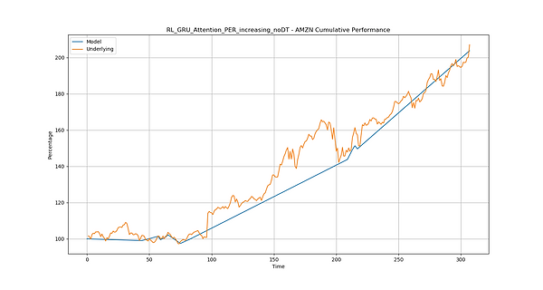
Model: RL_GRU_Attention_PER_increasing_noDT
-
Total Rewards 2839.583
-
Training Episode: 9
-
Num Parameter: 20786
-
Num Trading Day: 308
-
Num Year: 1.2
-
Num Trade: 26
-
Trade per Year: 21.666667
-
Win Ratio: 69.2254442%
-
Max Drawdown: -2.525205605%
-
Max Return: 103.7726721%
-
Sharpe Ratio: 3.892681198
-
Underlying Total Return: 107.0763109%
-
Underlying Annual Return: 83.4180264%
-
Model Total Return: 103.7726721%
-
Model Annual Return: 80.9762634
Graphical output:


Conclusion:
There were 3 new contributions in this project. Firstly, the improvement obtained with the new models compared to the other models was the main contribution. The GRU Attention with PER model outperformed the other RL models and the benchmark models in the test which included in different markets. This new combination could be used in many other domains to improve the model performance. The second contribution was the finding of the usefulness for the technical analysis tools in the RL models. Compared to the Huang 2018 paper where the Win Ratio obtained at most 63% and without the use of technical analysis tools, the new model could possibly get 74% Win Ratio with the use of the tools. The third contribution was the use of predefined markets in the study with a thorough EDA with the market data. The predefined markets were useful in the sense that they provide a clear reference for the report audiences and potential model users to access the model’s capabilities. It paved a way for easy comparison of the models.
Disclaimer: The model was still in academic research stage and only for demonstration. Investors can not use the above model to make investment decision.